Report Nips Style

\documentclass{article}

\usepackage[square, numbers]{natbib}
\bibliographystyle{elsarticle-harv}

% By default without options, the package will add line numbers and generate A4 size pages
% For preprint, pass "preprint". For anonymised submission, pass "anonymise". For letter size, pass "letter".
% To generate final version, pass "final".
% \usepackage{report_2019_JH}
% \usepackage[options1,options2]{report_2019_JH}

\usepackage[final,titlepage]{report_2019_JH}


% Packages imported in NIPS tex file
\usepackage[utf8]{inputenc}         % allow utf-8 input
\usepackage[T1]{fontenc}            % use 8-bit T1 fonts
\usepackage{hyperref}               % hyperlinks
\usepackage{url}                    % simple URL typesetting
\usepackage{booktabs}               % professional-quality tables
\usepackage{amsfonts}               % blackboard math symbols
\usepackage{nicefrac}               % compact symbols for 1/2, etc.
\usepackage{microtype}              % microtypography

% Other useful packages
\usepackage{float}
\usepackage{adjustbox}
\usepackage{amsmath}
\usepackage{amssymb}
\usepackage{array}
\usepackage{enumitem}               % allow roman-numbered lists
\usepackage{times}
\usepackage{longtable}
\usepackage{multirow}
\usepackage{xspace}
\usepackage{pgfgantt}
\usepackage{setspace}
%\doublespacing
\onehalfspacing

\DeclareRobustCommand{\eg}{e.g.\@\xspace}
\DeclareRobustCommand{\ie}{i.e.\@\xspace}

\makeatletter
\DeclareRobustCommand{\etc}{%
    \@ifnextchar{.}%
    {etc}%
    {etc.\@\xspace}%
}
\makeatother

% Table & texts commands
\newcolumntype{L}[1]{>{\raggedright\arraybackslash}p{#1}}
\newcolumntype{C}[1]{>{\centering\arraybackslash}p{#1}}

\newcolumntype{`}{>{\global\let\currentrowstyle\relax}}
\newcolumntype{~}{>{\currentrowstyle}}
\newcommand{\rowstyle}[1]{\gdef\currentrowstyle{#1}#1\ignorespaces }
\newcommand{\rbf}{\rowstyle{\bfseries}}

\newcommand{\norm}[1]{\left\lVert#1\right\rVert}
\newcommand{\gph}[2]{\includegraphics[width=#1\linewidth]{#2}}
\newcommand{\tbf}[1]{\textbf{#1}}
\newcommand{\tit}[1]{\textit{#1}}


\newcommand{\universityLogo}{images/logo1.png}              % Put university logo path here
\newcommand{\university}{My University / Faculty Name}      % Put university name here

\title{My Second Report}
\author{Your Name \\ \textit{ID / Some text}  \AND
        Co-author \\ \textit{Supervisor}      \AND
        Co-author \\ \textit{Co-supervisor}}

\begin{document}


\maketitle


\begin{abstract}
    An abstract paragraph. Lorem ipsum dolor sit amet, consectetur adipiscing elit. Maecenas pulvinar leo id felis pulvinar aliquet. Phasellus placerat dignissim odio aliquam hendrerit. Nullam vel justo eget ex feugiat congue. Pellentesque sagittis congue ipsum.
\end{abstract}


%-------------------------------------------------------------------------
%-------------------------------------------------------------------------
%-------------------------------------------------------------------------


\section{Introduction}
\label{sec: Introduction}

Nothing to introduce here. Just a collection of maths.



%-------------------------------------------------------------------------
%-------------------------------------------------------------------------
%-------------------------------------------------------------------------


\section{Products}
\label{sec: Products}

%-------------------------------------------------------------------------
\subsection{Inner product / Dot product}
\label{subsec: Inner product}

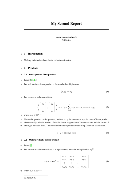
From \cite{wiki2019innerProd,wiki2019dotProd,wiki2019cosineSim}.

For real numbers, inner product is the standard multiplication:

\begin{equation}
    \langle x, y\rangle := x y
\end{equation}

For vectors or column matrices:

\begin{equation}
    \left\langle\left[ \begin{array}{c}{ x_{1}} \\ {\vdots} \\ {x_{n}}\end{array}\right], \left[ \begin{array}{c}{y_{1}} \\ {\vdots} \\ {y_{n}}\end{array}\right]\right\rangle := x^{T} y=\sum_{i=1}^{n} x_{i} y_{i}=x_{1} y_{1}+\cdots+x_{n} y_{n}
\end{equation}
\noindent
where $x, y \in\mathbb{R}\:^{n \times 1}$

The scalar product or dot product, written $x \cdot y$, is a common special case of inner product. Geometrically, it is the product of the Euclidean magnitudes of the two vectors and the cosine of the angle between them. These definitions are equivalent when using Cartesian coordinates. 

\begin{equation}
    \mathbf{x} \cdot \mathbf{y}=\|\mathbf{x}\|\|\mathbf{y}\| \cos \theta
\end{equation}


%-------------------------------------------------------------------------
\subsection{Outer product / Tensor product}
\label{subsec: Outer product}

From \cite{wiki2019outerProd}.

For vectors or column matrices, it is equivalent to a matrix multiplication $x y^{T}$:

\begin{equation}
    \mathbf{u} \otimes \mathbf{v} = \mathbf{u} \mathbf{v}^{T} = \left[ \begin{array}{cccc}{u_{1} v_{1}} & {u_{1} v_{2}} & {\ldots} & {u_{1} v_{n}} \\ {u_{2} v_{1}} & {u_{2} v_{2}} & {\dots} & {u_{2} v_{n}} \\ {\vdots} & {\vdots} & {\ddots} & {\vdots} \\ {u_{m} v_{1}} & {u_{m} v_{2}} & {\ldots} & {u_{m} v_{n}}\end{array}\right]
\end{equation}
\noindent
where $u, v \in\mathbb{R}\:^{n \times 1}$

For higher order tensors:

\begin{equation}
    \mathbf{T} = \mathbf{a} \otimes \mathbf{b} \otimes \mathbf{d}, \quad T_{i j k}=a_{i} b_{j} d_{k}
\end{equation}

For example, if $\mathbf{A}$ is of order $3$ with dimensions $(3, 5, 7)$ and $\mathbf{B}$ is of order $2$ with dimensions $(10, 100)$, their outer product $\mathbf{C}$ is of order $5$ with dimensions $(3, 5, 7, 10, 100)$.

Tensor product is a generalisation of outer product \cite{wiki2019tensorProd}. The outer product of two vectors $\mathbf{u}$ and $\mathbf{v}$ is their tensor product $\mathbf{u} \otimes \mathbf{v}$ \cite{wiki2019outerProd}.


%-------------------------------------------------------------------------
\subsection{Hadamard product}
\label{subsec: Hadamard product}

From \cite{wiki2019hadamardProd}.

The Hadamard product (also known as the Schur product or the entrywise product) is a binary operation that takes two matrices of the same dimensions and produces another matrix where each element $i, j$ is the product of elements $i, j$ of the original two matrices. 

For two matrices $\mathbf{A}$ and $\mathbf{B}$ of the same dimension $m \times n$, the Hadamard product $\mathbf{A} \circ \mathbf{B}$ is a matrix of the same dimension as the operands:

\begin{equation}
    (A \circ B)_{i j}=(A)_{i j}(B)_{i j}
\end{equation}

For example:

\begin{equation}
    \left[ \begin{array}{ccc}{a_{11}} & {a_{12}} & {a_{13}} \\ {a_{21}} & {a_{22}} & {a_{23}} \\ {a_{31}} & {a_{32}} & {a_{33}}\end{array}\right] \circ \left[ \begin{array}{ccc}{b_{11}} & {b_{12}} & {b_{13}} \\ {b_{21}} & {b_{22}} & {b_{23}} \\ {b_{31}} & {b_{32}} & {b_{33}}\end{array}\right]=\left[ \begin{array}{ccc}{a_{11} b_{11}} & {a_{12} b_{12}} & {a_{13} b_{13}} \\ {a_{21} b_{21}} & {a_{22} b_{22}} & {a_{23} b_{23}} \\ {a_{31} b_{31}} & {a_{32} b_{32}} & {a_{33} b_{33}}\end{array}\right]
\end{equation}


%-------------------------------------------------------------------------
\subsection{Circular correlation}
\label{subsec: Circular correlation}

From \cite{nickel2016holographic,plate1995holographic}, related: \cite{tay2017learning}.

Circular correlation between two vectors $\mathbf{a} \star \mathbf{b}$ is defined as:

\begin{equation}
    y_k = \left[\mathbf{c} \star \mathbf{t}\right]_{k} = \sum_{i=0}^{d-1} c_{i} \, t_{(k+i) \bmod d} \qquad \text{for} \; i = 0, \dotsc, d-1
\end{equation}
\noindent
where $\star : \mathbb{R}^{d} \times \mathbb{R}^{d} \rightarrow \mathbb{R}^{d}$

\begin{figure}[h]
\begin{minipage}{0.5\linewidth}
    \begin{center}
    \gph{0.5}{images/circular_correlation.png}
    \end{center}
\end{minipage}
\begin{minipage}{0.5\linewidth}
    \begin{equation}
        \begin{array}{c}{\mathbf{y} = \mathbf{c} \star \mathbf{t}} \\ {y_{0}=c_{0} t_{0}+c_{1} t_{1}+c_{2} t_{2}} \\ {y_{1}=c_{2} t_{0}+c_{0} t_{1}+c_{1} t_{2}} \\ {y_{2}=c_{1} t_{0}+c_{2} t_{1}+c_{0} t_{2}}\end{array}
    \end{equation}
\end{minipage}
\caption{Circular correlation. Figure from \cite{plate1995holographic}, equations from \cite{plate1995holographic,nickel2016holographic}.}
\end{figure}

Properties include:

\begin{enumerate}[label=\roman*)]
    \item {\tbf{Non Commutative} \\
            Correlation, unlike convolution, is not commutative, \ie{} $\mathbf{a} \star \mathbf{b} \neq \mathbf{b} \star \mathbf{a}$. Non-commutativity is necessary to model asymmetric relations (directed graphs).}
    \item {\tbf{Similarity Component} \\
            In the correlation $\mathbf{a} \star \mathbf{b}$, a single component $[\mathbf{a} \star \mathbf{b}]_{0}=\sum_{i} a_{i} b_{i}$ corresponds to the dot product $\langle\mathbf{a}, \mathbf{b}\rangle$. The existence of such a component can be helpful to model relations in which the similarity of entities is important. No such component exists in circular convolution $\mathbf{a} \circledast \mathbf{b}$.}
\end{enumerate}


%-------------------------------------------------------------------------
\subsection{Circular convolution}
\label{subsec: Circular convolution}

From \cite{plate1995holographic,nickel2016holographic,dubois2017working}.

\begin{equation}
    t_k = \left[\mathbf{c} \circledast \mathbf{x}\right]_{k} = \sum_{i=0}^{d-1} c_{i} \, x_{(k-i) \bmod d} \qquad \text{for} \; i = 0, \dotsc, d-1
\end{equation}
\noindent
where $\circledast : \mathbb{R}^{d} \times \mathbb{R}^{d} \rightarrow \mathbb{R}^{d}$


\begin{figure}[h]
\begin{minipage}{0.5\linewidth}
    \begin{center}
    \gph{0.5}{images/circular_convolution.png}
    \end{center}
\end{minipage}
\begin{minipage}{0.5\linewidth}
    \begin{equation}
        \begin{array}{c}{\mathbf{t} = \mathbf{c} \circledast \mathbf{x}} \\ {t_{0}=c_{0} x_{0}+c_{2} x_{1}+c_{1} x_{2}} \\ {t_{1}=c_{1} x_{0}+c_{0} x_{1}+c_{2} x_{2}} \\ {t_{2}=c_{2} x_{0}+c_{1} x_{1}+c_{0} x_{2}}\end{array}
    \end{equation}
\end{minipage}
\caption{Circular convolution. Figure and equations from \cite{plate1995holographic}.}
\end{figure}

Properties include:

\begin{enumerate}[label=\roman*)]
    \item {\tbf{Commutative} \\
                Convolution (cyclic or acyclic) is commutative, \ie{} $\mathbf{a} \circledast \mathbf{b} = \mathbf{b} \circledast \mathbf{a}$.}
\end{enumerate}



%-------------------------------------------------------------------------
%-------------------------------------------------------------------------
%-------------------------------------------------------------------------


\clearpage
\singlespacing

%\renewcommand\refname{Bibliography}
\bibliography{ref}
\end{document}